绘制颜色直方图

背景
1. 获取图像颜色通道数据
2. 绘制颜色直方图
总结
附录

背景

一个可视化图表是怎么画出来的？这是一个既复杂又简单的问题。复杂在于，笔者整理过、有专有名字的可视化图表就有数百上千种，每一种或多或少都不太一样，要穷举起来是一项艰难的工作。简单在于，万变不离其宗，至少绘制一个二维平面下的统计类图表，有非常标准的几个步骤，每一个步骤用前端实现起来都只有寥寥百来行代码而已。本文将带大家在不依赖任何第三方绘图库的情况下，把非常常用的一种可视化图表--颜色直方图，在浏览器里画出来。

颜色直方图（color histogram），是图像处理（image processing）领域的基础概念。简单来说就是用直方图表达一张图片（RGB）三个颜色的通道值分布情况。它在图像处理、图像识别、图像检索等方面的应用都很广。绘制颜色直方图，将会涉及到大部分统计图表绘制所必需的数据准备、数据处理、数据映射、绘图的完整流程。接下来我们一步一步将下面图像（左）对应的直方图（右）画出来。

CV 领域著名的“lena”图

对应直方图

1. 获取图像颜色通道数据

图像在前端的表现形式是一个 8 位数字（2^8）的数组（Unit8ClampedArray），数组里每个元素代表一个颜色通道值（0-255）。这些颜色通道的值都是扁平存储到一起的，也就是[r0, g0, b0, a0, r1, g1, b1, a1, ...] 这样的形式。

获取这个 Unit8ClampedArray 的方式有两种，一种直接从 canvas 实例里获取：

const ctx = canvasElement.getContext('2d')
const { width, height } = canvasElement
const image = ctx.getImageData(0, 0, width, height)
return image.data

另一个方式是从 Image 实例获取，这时候需要先自行生成 canvas 实例，写入图片数据，再导出：

const canvas = document.createElement('canvas')
const ctx = canvas.getContext('2d')
const myImgElement = document.getElementById('foo')
ctx.drawImage(myImgElement, 0, 0)
const { width, height } = myImgElement
const image = ctx.getImageData(0, 0, width, height)
return image.data

这样获取到的数组就是我们在前端（浏览器端）做图像处理的核心数据。要获取图片的颜色直方图，我们需要先遍历这个数组，拿到 RGB 三个颜色通道的所有值（0-255）。

const rs = []
const gs = []
const bs = []
for (let i = 0; i < data.length; i += 4) {
  rs.push(data[i])
  gs.push(data[i + 1])
  bs.push(data[i + 2])
}

目前为止我们拿到了三个颜色通道在图像上的所有值，这就是用于绘制颜色直方图的原始数据。下一步就是根据这个原始数据进行处理和绘图。

2. 绘制颜色直方图

怎么画一张直方图（histogram）呢？绘制传统直方图拢共分五步：

数据分箱
数据度量（获取分箱值和概率值的值域范围、坐标标度等）
数据映射到实际绘图属性（位置、形状、颜色等）
绘制几何图形
~~绘制坐标轴、图例、标题（TODO）~~

什么是分箱（binning）？所谓分箱是数据分析领域很重要的概念，是数据预处理的一环。对于连续型数据，我们实际数据来源可能会有很多异常值、噪音等，像“重 56.21kg”这样的数据，虽然精准，但从统计的角度看是不利于分析发现规律的。例如我们想要统计一个拳击比赛的选手体重分布，通常希望得到的是：45 到 50 公斤级的人数、50 到 55 公斤级的人数等，原始数据需要“放到一个区间里”，才进行下一步的统计分析。

传统直方图表达的就是“在各个值域区间的值分布情况”。它主要传达的信息就是连续性数据的概率分布。应用到图像的颜色上，传达的信息就是各个颜色通道的分布规律。例如上述 lena 图像的颜色直方图可以看到，“高光部分偏红，暗部偏绿”，因为红色大部分集中在 [128, 255] 区间，而绿色集中在 [0, 128]区间。应用分箱，我们可以从不同的粒度去看概率分布（自上而下分箱区间宽度分别是 20、10、5、2、1）：

binWidth=20

binWidth=10

binWidth=5

binWidth=2

binWidth=1

直方图分箱算法的核心流程很简单：先根据给定数据的极值（min、max）以及分箱区间宽度（或者分箱数量），把要分箱的值域分割成具体分箱的区间。然后遍历所有数据，每个数据用二分搜索定位到具体的分箱中，最后得到类似这样的数据结构：

const rBins = [
  {
    x0: 0,
    x1: 10,
    values: [0, 0 /* ... */, , 10, 10, 10],
    count: 51,
  } /* ... */,
]

分箱后的数据就可以明显看到和最终可视化图形的对应关系了。x 轴就是区间值，亦即分箱数据里的 x0 和 x1。y 轴就是在这个分箱区间内数据出现的次数 count。接下来的问题就是如何把真实的分箱数据映射成可视化图形里的绘图属性了。譬如 x0、x1 在图里具体要画到哪一像素？count 是 40 和 400，在图中要画多高，具体多少像素？

在具体画图之前还有一个最关键的步骤，就是获取数据度量（scale）。数据度量在可视化里是最关键最核心的模块。它本质的使命就是分析原始数据 domain 的特征，并且把原始数据空间映射到图形空间，从而能把数据“画出来”。此外，它还肩负计算坐标轴间距、标签值等任务。

Leland Wilkinson wrote in book "The Grammar of Graphics"

If we endeavor to develop a charting instead of a graphing program, we will accomplish two things. First, we inevitably will offer fewer charts than people want. Second, our package will have no deep structure. Our computer program will be unnecessarily complex, because we will fail to reuse objects or routines that function similarly indifferent charts. And we will have no way to add new charts to our system without generating complex new code. Elegant design requires us to think about a theory of graphics, not charts.

连续变量的 scale 模块核心功能是两部分：一部分是数据 mapping（正向 transform，反向 transform）；一部分是 nice labeling（获得易读的坐标轴标签）。大体的类设计是这样的：

const unit = [0, 1]
class ContinuousScale {
  domain = unit
  range = unit
  ticks = []
  constructor(domain, range) {}
  transform(x, isInvert = false) {
    // 把 domain 值域中的值转换到 range 值域，或者反过来
  }
  scale(x) {
    return this.transform(x)
  }
  invert(x) {
    return this.transform(x, true)
  }
  niceLabeling() {}
}

其中，domain 不一定只有一对 [min, max] 组合，有可能和分箱一样，是多个区间。range 亦然。因此做值转换的时候，先要通过二分搜索定位到一个区间，再根据映射规则（最常见的是线性映射）转换到对应的值。

另外，nice labeling 也是个很有意思的话题。我们希望看到的“好看”的坐标轴标签，通常是符合一定规律的。wilkinson 的思路就是符合 [1, 5, 2, 2.5, 4, 3] 这些倍数关系的值，譬如 0, 100, 200 这样的标签是人比较易读的标签。算法实现做了 r-pretty 和 wilkinson-extended 两个算法，感兴趣的同学可以研究一下附录的源码。

有了 scale 模块，我们就可以把原始数据 (x0, x1, count) 映射到图形属性 (x, y) 上了。domain 就是 bins 里的 x0, x1, count 这些数据，range 就是绘图画布上的宽 width、高 height。按照传统直方图的画法，每个分箱（bin）是一个矩形，用 SVG 来表示图形属性可以这么画：

function bins2paths(bins, xScale, yScale) {
  return bins
    .map((_bin) => {
      const x0 = xScale.scale(_bin.x0)
      const x1 = xScale.scale(_bin.x1)
      const y0 = yScale.scale(0)
      const y1 = yScale.scale(_bin.count)
      return `<path d="M${x0} ${y0}L${x0} ${y1}L${x1} ${y1}L${x1} ${y0}Z"/>`
    })
    .join('\n')
}

思路其实就是用 L 指令 line to 的形式连接四个顶点。最终可以得出这样的结果：

这里要注意一个点：SVG 的绘图是从左上角 (0, 0) 开始往右、往下画的，但我们的可视化图表不是的。可视化图表正常是用笛卡尔坐标系，x 轴从左到右是从 0 到 width，但 y 轴是从下到上，因而是和 SVG 绘图相反的。所以 yScale 的设定我们需要做一下处理，domain 是 0 到 maxCount，但 range 应该是从 height 到 0（反向）。这样绘制出来的结果就是正常笛卡尔坐标系的感觉了。

另外整体 SVG 结构如下，这里还利用了 g 标签分组继承绘图属性的特性。

return `<svg viewBox="0 0 ${w} ${h}" xmlns="http://www.w3.org/2000/svg">
  <g class="background">
    <rect x="0" y="0" width="${w}" height="${h}" fill="white" stroke="grey" stroke-width="1"/>
  </g>
  <g class="grid"><!-- TODO --></g>
  <g class="graph" stroke-width="1">
    <g class="histogram red" stroke="#f00" fill="rgba(255,0,0,0.5)">
      ${bins2paths(rBins, xScale, yScale)}
    </g>
    <g class="histogram green" stroke="#0f0" fill="rgba(0,255,0,0.5)">
      ${bins2paths(gBins, xScale, yScale)}
    </g>
    <g class="histogram blue" stroke="#00f" fill="rgba(0,0,255,0.5)">
      ${bins2paths(bBins, xScale, yScale)}
    </g>
  </g>
  <g class="components">
    <g class="axes">
      <!-- TODO -->
      <g class="axis axis-x"></g>
      <g class="axis axis-y"></g>
    </g>
  </g>
</svg>`

对于图像的颜色直方图而言，传统直方图的展示效果其实并不好，虽然精确，但信息密度比较高，不够“圆润美观”。所以另一个选择是用面积图（带填充颜色的曲线图）来画。

function bins2path(bins, xScale, yScale) {
  const minX = xScale.scale(xScale.domain[0])
  const maxX = xScale.scale(xScale.domain[1])
  const minY = yScale.scale(yScale.domain[0])
  const points = bins.map((_bin) => [xScale.scale(_bin.x0), yScale.scale(_bin.count)])
  const first = points.shift()
  return `<path d="M${minX},${minY}L${first[0]} ${first[1]}L${points
    .map((p) => `${p[0]},${p[1]}`)
    .join('L')}L${maxX},${minY}Z"/>`
}

这个方法关键在于用 L 指令，连接各个分箱顶点，以统一的色块表达整体分布效果，会比“多个柱子集合”的形式更圆润和直观一些。

至此我们已经得到一个可以洞察图像颜色分布信息的颜色直方图。使用这个方案后，后续还有不少事情可以做：

补全坐标轴信息（x 轴就是 0 到 255，y 轴加上 label 可以获取更精准的“数量分布”）
性能优化

第 1 点暂缓，第 2 点涉及一个比较有意思的点：line simplification。对于图像的颜色直方图而言，一个颜色通道固定会有 255 个点。如果画布比较大，我们应当展示全部的信息；但如果画布很小，我们要考虑简化，否则点挤到一起密密麻麻会影响美观度和信息传达。

这个步骤使用的算法也是非常成熟的算法，算法核心就是看临近三个点连线形成的夹角，夹角很大，那代表中间的点弯折很大，是关键点，如果夹角很小，那中间点就可以忽略。感兴趣的同学可以研究一下附录的源码。

后续的工作，除了可以为直方图补充好坐标轴、刻度、标题、Tooltip 等辅助组件以外，还有一个特别有意思的优化：现在的图看起来像是曲线，但其实是“折线”，怎么样把折线变成“准确的曲线”？SVG 里绘制曲线的指令是 C（三阶贝塞尔曲线，也包含 S 指令）或者 Q（二阶贝塞尔曲线，也包含 T 指令），应该如何在原有折线的基础上补充相关控制点，让它真正变成“圆润而准确的曲线”？这也是一个相当有挑战的问题，留待感兴趣的读者深入挖掘下去。

总结

CV 和 Data Vis 都是很古老的领域，这些领域里我们能看到非常成熟的工程体系，大部分前人的工作，已经不仅仅考虑工程实现层面的架构了，而更下探到了理论层面。“为了做好这件事，从理论框架上我们能做什么样的抽象，使得上层应用实现具有更好的灵活度和可维护性？”。像可视化，已经抽象到“数学空间映射”这个程度了。不过在前端方向，经典理论成熟的体系，往往在 web 层面还是蓝海，还没有对应的、高质量的工程实现。这对于我们是非常好的机会，我们可以结合领域沉淀和前端技术，真的为无限的交互场景带来首创性的技术红利。

附录

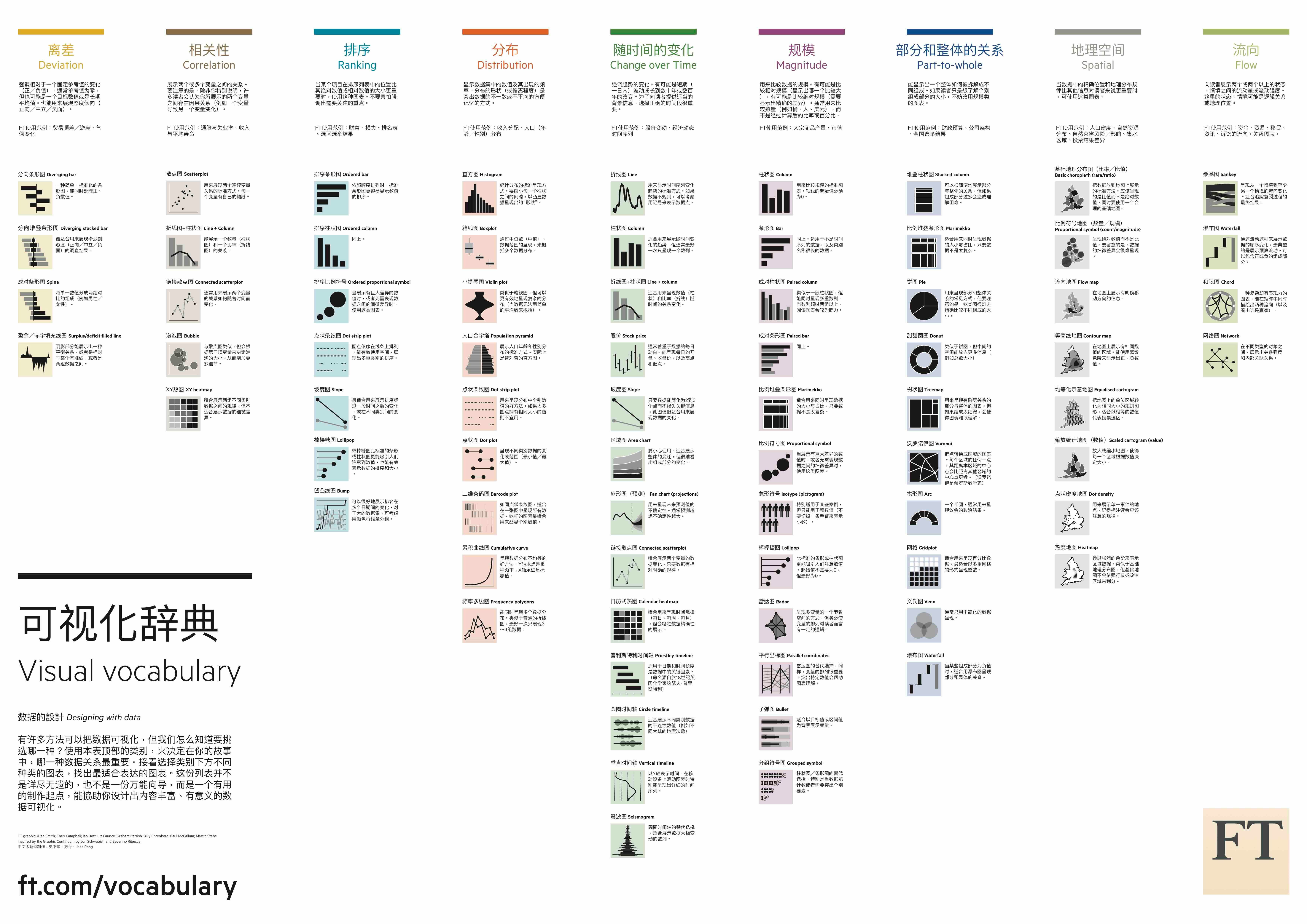
one more thing: visual vocabulary

在多个流程中涉及的“二分搜索”实现

function bisectLeft(arr, x, lo, hi) {
  if (isNil(lo)) lo = 0
  if (isNil(hi)) hi = arr.length
  while (lo < hi) {
    const mid = Math.floor((lo + hi) / 2)
    if (x > arr[mid]) lo = mid + 1
    else hi = mid
  }
  return lo
}

nice labeling 算法实现

r-pretty

/*
R pretty:
https://svn.r-project.org/R/trunk/src/appl/pretty.c
https://www.rdocumentation.org/packages/base/versions/3.6.2/topics/pretty
*/
const {
  DBL_EPSILON,
  DBL_MAX,
  DBL_MIN,
} = require('../constants');

function rPretty(
  min = 0, max = 0,
  nDiv = 5, minN = 0,utils
  shrinkSml = 0.75,
  h = 1.5, h5 = (0.5 + 1.5 * 1.5),
  epsCorrect = 0,
  returnBounds = true,
) {
  const roundingEps = 1e-10;
  const dx = max - min;
  let isSmall = false;
  let cell;
  let u;
  if (dx === 0 && min === 0) {
    /* cell is "scale" */
    cell = 1;
    isSmall = true;
  } else {
    cell = (Math.abs(min), Math.abs(max));
    u = 1 + ((h5 >= 1.5 * h + 0.5) ? 1 / (1 + h) : 1.5 / (1 + h5));
    u *= Math.max(1, nDiv) * DBL_EPSILON; // avoid overflow for large nDiv
    /* added times 3, as several calculations here */
    isSmall = dx < cell * u * 3;
  }

  // small numbers
  if (isSmall) {
    if (cell > 10) cell = 9 + cell / 10;
    cell *= shrinkSml;
    if (minN > 1) cell /= minN;
  } else {
    cell = dx;
    if (nDiv > 1) cell /= nDiv;
  }

  if (cell < 20 * DBL_MIN) {
    console.warn('vary small range corrected');
    cell = 20 * DBL_MIN;
  } else if (cell * 10 > DBL_MAX) {
    console.warn('vary large range corrected');
    cell = 0.1 * DBL_MAX;
  }

  const base = 10 ** Math.floor(Math.log10(cell)); /* base <= cell < 10 * base */
  /** unit: from [1, 2, 5, 10] * base
   * such that |u - cell\ is small
   * favoring larger (if h > 1, else smaller) u values
   * favor '5' more than '2', if h5 > h (default h5 = 0.5 + 1.5h)
   */
  let unit = base;
  u = 2 * base;
  if (u - cell < h * (cell - unit)) {
    unit = u;
    u = 5 * base;
    if (u - cell < h5 * (cell - unit)) {
      unit = u;
      u = 10 * base;
      if (u - cell < h * (cell - unit)) {
        unit = u;
      }
    }
  }
  /** Result: c := cell,  u := unit,  b := base
   * c in [1,(2+ h) /(1+h)] b ==> u=  b
   * c in ( (2+ h)/(1+h),  (5+2h5)/(1+h5)] b ==> u= 2b
   * c in ( (5+2h)/(1+h), (10+5h) /(1+h) ] b ==> u= 5b
   * c in ((10+5h)/(1+h), 10) b ==> u=10b
   * ===> 2/5 *(2+h)/(1+h) <= c/u <= (2+h)/(1+h)
   */
  let ns = Math.floor(min / unit + roundingEps);
  let nu = Math.ceil(max / unit - roundingEps);

  if (epsCorrect && (epsCorrect > 1 || !isSmall)) {
    if (min !== 0) min *= (1 - DBL_EPSILON);
    else min = -DBL_MIN;

    if (max !== 0) max *= (1 + DBL_EPSILON);
    else max = +DBL_MIN;
  }

  while (ns * unit > min + roundingEps * unit) ns -= 1;
  while (nu * unit < max - roundingEps * unit) nu += 1;

  let k = parseInt(0.5 + nu - ns, 10);
  if (k < minN) {
    k = minN - k;
    if (ns >= 0) {
      nu += k / 2;
      ns -= k / 2 + (k % 2);
    } else {
      ns -= k / 2;
      nu += k / 2 + (k % 2);
    }
    nDiv = minN;
  } else {
    nDiv = k;
  }

  if (returnBounds) {
    if (ns * unit < min) min = ns * unit;
    if (nu * unit > max) max = nu * unit;
  } else {
    min = ns;
    max = nu;
  }

  const res = {
    min,
    max,
    ticks: [],
  };
  const toFixed = base < 1 ? Math.ceil(Math.abs(Math.log10(base))) : 0;
  let x = Number.parseFloat((ns * unit).toFixed(toFixed));
  while (x < max) {
    res.ticks.push(x);
    x += unit;
    if (toFixed) {
      x = Number.parseFloat(x.toFixed(toFixed));
    }
  }
  res.ticks.push(x);
  return res;
}

module.exports = rPretty;

wilkonson-extended

const { isNumber, modulo } = require('../../utils')

const DEFAULT_Q = [1, 5, 2, 2.5, 4, 3]
// const ALL_Q = [1, 5, 2, 2.5, 4, 3, 1.5, 7, 6, 8, 9];
const eps = Number.EPSILON * 100

function simplicity(q, Q, j, lmin, lmax, lstep) {
  const n = Q.length
  const i = Q.indexOf(q)
  let v = 0
  const m = modulo(lmin, lstep)
  if ((m < eps || lstep - m < eps) && lmin <= 0 && lmax >= 0) {
    v = 1
  }
  return 1 - i / (n - 1) - j + v
}
function simplicityMax(q, Q, j) {
  const n = Q.length
  const i = Q.indexOf(q)
  const v = 1
  return 1 - i / (n - 1) - j + v
}
function density(k, m, dmin, dmax, lmin, lmax) {
  const r = (k - 1) / (lmax - lmin)
  const rt = (m - 1) / (Math.max(lmax, dmax) - Math.min(dmin, lmin))
  return 2 - Math.max(r / rt, rt / r)
}
function densityMax(k, m) {
  if (k >= m) return 2 - (k - 1) / (m - 1)
  return 1
}
function coverage(dmin, dmax, lmin, lmax) {
  const range = dmax - dmin
  return 1 - (0.5 * ((dmax - lmax) ** 2 + (dmin - lmin) ** 2)) / (0.1 * range) ** 2
}
function coverageMax(dmin, dmax, span) {
  const range = dmax - dmin
  if (span > range) {
    const half = (span - range) / 2
    return 1 - half ** 2 / (0.1 * range) ** 2
  }
  return 1
}
function legibility() {
  return 1
}

/**
 * An Extension of Wilkinson's Algorithm for Position Tick Labels on Axes
 * https://www.yuque.com/preview/yuque/0/2019/pdf/185317/1546999150858-45c3b9c2-4e86-4223-bf1a-8a732e8195ed.pdf
 * @param dmin min number
 * @param dmax max number
 * @param m count for ticks
 * @param onlyLoose can min / max be extended
 * @param Q nice numbers set
 * @param w weights for 4 components
 */
module.exports = function extended(
  dmin,
  dmax,
  m = 5,
  onlyLoose = true,
  Q = DEFAULT_Q,
  w = [0.25, 0.2, 0.5, 0.05]
) {
  // exceptions
  if (!isNumber(dmin) || !isNumber(dmax)) {
    return {
      min: 0,
      max: 0,
      ticks: [],
    }
  }
  if (dmin === dmax || m === 1) {
    return {
      min: dmin,
      max: dmax,
      ticks: [dmin],
    }
  }

  const best = {
    score: -2,
    lmin: 0,
    lmax: 0,
    lstep: 0,
  }
  let j = 1
  while (j < Infinity) {
    for (let i = 0; i < Q.length; i += 1) {
      const q = Q[i]
      const sm = simplicityMax(q, Q, j)
      if (Number.isNaN(sm)) {
        throw new Error('NaN')
      }
      if (w[0] * sm + w[1] + w[2] + w[3] < best.score) {
        j = Infinity
        break
      }
      let k = 2
      while (k < Infinity) {
        const dm = densityMax(k, m)
        if (w[0] * sm + w[1] + w[2] * dm + w[3] < best.score) {
          break
        }

        const delta = (dmax - dmin) / (k + 1) / j / q
        let z = Math.ceil(Math.log10(delta))

        while (z < Infinity) {
          const step = j * q * 10 ** z
          const cm = coverageMax(dmin, dmax, step * (k - 1))

          if (w[0] * sm + w[1] * cm + w[2] * dm + w[3] < best.score) {
            break
          }

          const minStart = Math.floor(dmax / step) * j - (k - 1) * j
          const maxStart = Math.ceil(dmin / step) * j

          if (minStart > maxStart) {
            z += 1
            /* eslint-disable-next-line no-continue */
            continue
          }
          for (let start = minStart; start <= maxStart; start += 1) {
            const lmin = start * (step / j)
            const lmax = lmin + step * (k - 1)
            const lstep = step

            const s = simplicity(q, Q, j, lmin, lmax, lstep)
            const c = coverage(dmin, dmax, lmin, lmax)
            const g = density(k, m, dmin, dmax, lmin, lmax)
            const l = legibility()

            const score = w[0] * s + w[1] * c + w[2] * g + w[3] * l
            if (score > best.score && (!onlyLoose || (lmin <= dmin && lmax >= dmax))) {
              best.lmin = lmin
              best.lmax = lmax
              best.lstep = lstep
              best.score = score
            }
          }
          z += 1
        } // end of z-while-loop
        k += 1
      } // end of k-while-loop
    }
    j += 1
  }
  // get fixed numbers
  const toFixed = Number.isInteger(best.lstep) ? 0 : Math.ceil(Math.abs(Math.log10(best.lstep)))
  const range = []
  for (let tick = best.lmin; tick <= best.lmax; tick += best.lstep) range.push(tick)
  const ticks = toFixed ? range.map((x) => Number.parseFloat(x.toFixed(toFixed)), 10) : range
  return {
    min: Math.min(dmin, ticks[0]),
    max: Math.max(dmax, ticks[ticks.length - 1]),
    ticks,
  }
}

line-simplification 算法实现

// Point format: [x, y]
function getSqDist(p1, p2) {
  const dx = p1[0] - p2[0]
  const dy = p1[1] - p2[1]
  return dx * dx + dy * dy
}

function getSqSegDist(p, p1, p2) {
  let [x, y] = p1
  let dx = p2[0] - x
  let dy = p2[1] - y

  if (dx !== 0 || dy !== 0) {
    const t = ((p[0] - x) * dx + (p[1] - y) * dy) / (dx * dx + dy * dy)
    if (t > 1) {
      x = p2[0]
      y = p2[1]
    } else if (t > 0) {
      x += dx * t
      y += dy * t
    }
  }
  dx = p[0] - x
  dy = p[1] - y
  return dx * dx + dy * dy
}

// basic distance-based simplification
function simplifyRadialDist(points, sqTolerance) {
  let prevPoint = points[0]
  const newPoints = [prevPoint]
  let point

  for (let i = 1, len = points.length; i < len; i += 1) {
    point = points[i]
    if (getSqDist(point, prevPoint) > sqTolerance) {
      newPoints.push(point)
      prevPoint = point
    }
  }
  if (prevPoint !== point) newPoints.push(point)
  return newPoints
}

function simplifyDPStep(points, first, last, sqTolerance, simplified) {
  let maxSqDist = sqTolerance
  let index

  for (let i = first + 1; i < last; i += 1) {
    const sqDist = getSqSegDist(points[i], points[first], points[last])
    if (sqDist > maxSqDist) {
      index = i
      maxSqDist = sqDist
    }
  }
  if (maxSqDist > sqTolerance) {
    if (index - first > 1) simplifyDPStep(points, first, index, sqTolerance, simplified)
    simplified.push(points[index])
    if (last - index > 1) simplifyDPStep(points, index, last, sqTolerance, simplified)
  }
}

// simplification using Ramer-Douglas-Peucker algorithm
function simplifyDouglasPeucker(points, sqTolerance) {
  const last = points.length - 1
  const simplified = [points[0]]
  simplifyDPStep(points, 0, last, sqTolerance, simplified)
  simplified.push(points[last])
  return simplified
}

// both algorithms combined for awesome performance
module.exports = function simplify(points, tolerance, highestQuality) {
  if (points.length <= 2) return points
  const sqTolerance = tolerance !== undefined ? tolerance * tolerance : 1
  points = highestQuality ? points : simplifyRadialDist(points, sqTolerance)
  points = simplifyDouglasPeucker(points, sqTolerance)
  return points
}